

I’d like to do a song of great social and political import.
The code that created the illustrations in Tao Te Programming is now available as the TaoTeProgramming package on CRAN.
The sea is just flat hills
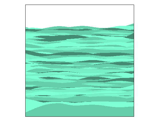
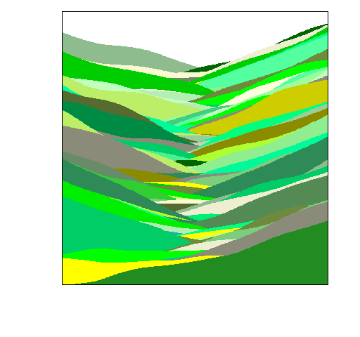 And they are both just smooth mountains.
The package contains just over 1000 lines of code. More than half of that is the functions that create the specific pictures in the book. All of the real functionality is produced with about 450 lines of R.
You might think this is because I followed the principles in Chapter 21 to get complexity by writing simple code. Actually it comes from laziness (Chapter 26) — if something wasn’t working well with minimal effort, I threw it out. Mostly it’s randomness that’s the powerhouse.
One call to make them all
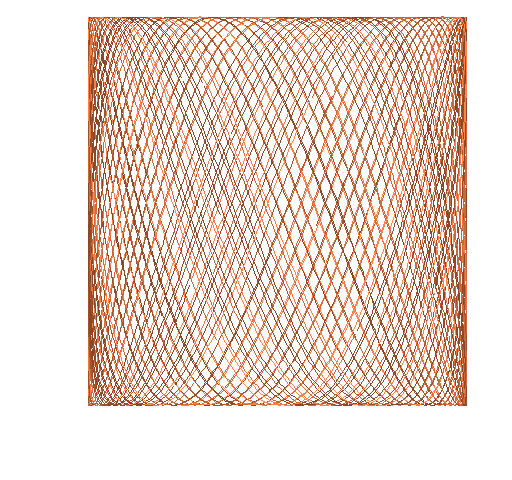
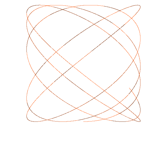
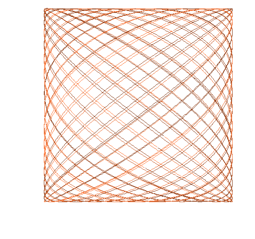
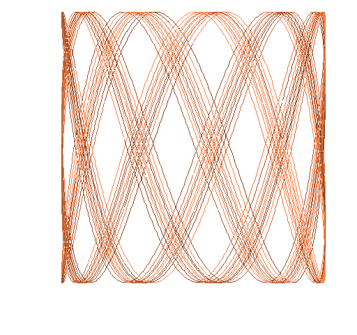
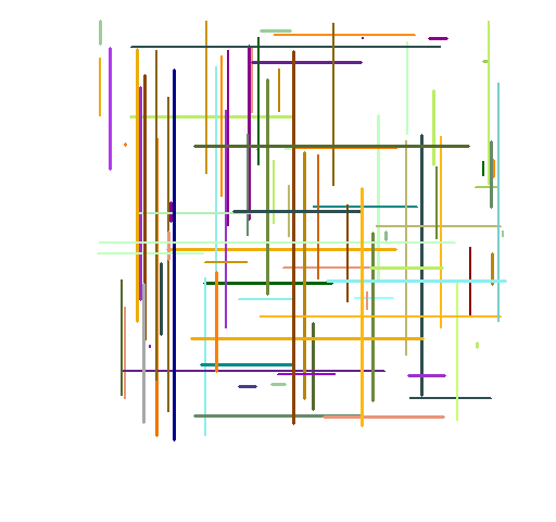
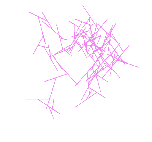
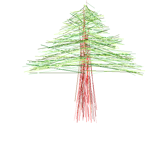
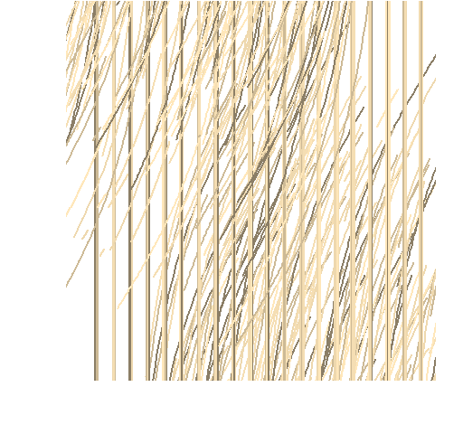
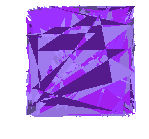
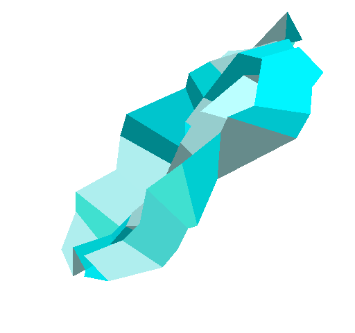
The next 6 figures are all produced by the exact same code. The only difference is the random seed that is used.
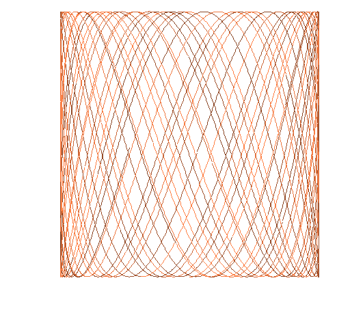
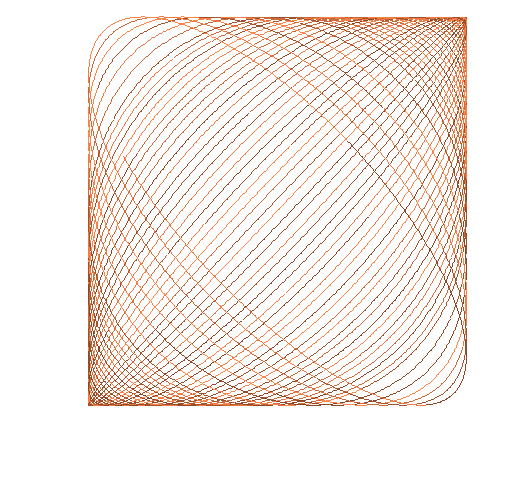
 Yet more

This post comes under the domain of Chapter 65: Play.
Epilogue
That’s it. He-he-he …
— Janis Joplin
Appendix R
Here are the functions (in no particular order) that produce the pictures above (WordPress is not especially good at preserving the formatting).
require(TaoTeProgramming)

P.polytilepurple14 <- function (filename = "polytilepurple14.png")
{
 if(length(filename)) {
 png(file=filename, width=512)
 par(mar=c(4,5, 0, 2) + .1)
 }
 polytile(color=grep("purple", colors(), value=TRUE), seed=14)

 if(length(filename)) {
 dev.off()
 }
}

P.quadtileorange4 <- function (filename = "quadtileorange4.png")
{
 if(length(filename)) {
 png(file=filename, width=512)
 par(mar=c(4,5, 0, 2) + .1)
 }
 quadtile(color=grep("orange", colors(), value=TRUE),
 dims=c(2,20), seed=4)

 if(length(filename)) {
 dev.off()
 }
}

P.qtbalturquoise37 <- function (filename = "qtbalturquoise37.png")
{
 if(length(filename)) {
 png(file=filename, width=512)
 par(mar=c(4,5, 0, 2) + .1)
 }
 quadtilebalance(color=grep("turquoise", colors(), value=TRUE),
 seed=37)

 if(length(filename)) {
 dev.off()
 }
}

P.darkroad1 <- function (filename = "darkroad1.png")
{
 if(length(filename)) {
 png(file=filename, width=512)
 par(mar=c(4,5, 0, 2) + .1)
 }
 roads(color=grep("dark", colors(), value=TRUE), lwd=2:3, seed=1)

 if(length(filename)) {
 dev.off()
 }
}

P.wheatwave9 <- function (filename = "wheatwave9.png")
{
 if(length(filename)) {
 png(file=filename, width=512)
 par(mar=c(4,5, 0, 2) + .1)
 }
 waves(color=grep("wheat", colors(), value=TRUE),
 lwd=2, seed=9)

 if(length(filename)) {
 dev.off()
 }
}

P.violetstick54 <- function (filename = "violetstick54.png")
{
 if(length(filename)) {
 png(file=filename, width=512)
 par(mar=c(4,5, 0, 2) + .1)
 }
 sticks(color="violet", lwd=2, seed=54)

 if(length(filename)) {
 dev.off()
 }
}

P.bendsienna0 <- function (filename = "bendsienna0.png")
{
 if(length(filename)) {
 png(file=filename, width=512)
 par(mar=c(4,5, 0, 2) + .1)
 }
 bendplotmultcol(xdelta=100, ydelta=200, sd=.001,
 color=grep("sienna", colors(), value=TRUE),
 seed=0)

 if(length(filename)) {
 dev.off()
 }
}

P.bendsienna1 <- function (filename = "bendsienna1.png")
{
 if(length(filename)) {
 png(file=filename, width=512)
 par(mar=c(4,5, 0, 2) + .1)
 }
 bendplotmultcol(xdelta=100, ydelta=200, sd=.001,
 color=grep("sienna", colors(), value=TRUE),
 seed=1)

 if(length(filename)) {
 dev.off()
 }
}

P.bendsienna2 <- function (filename = "bendsienna2.png")
{
 if(length(filename)) {
 png(file=filename, width=512)
 par(mar=c(4,5, 0, 2) + .1)
 }
 bendplotmultcol(xdelta=100, ydelta=200, sd=.001,
 color=grep("sienna", colors(), value=TRUE),
 seed=2)

 if(length(filename)) {
 dev.off()
 }
}

P.bendsienna3 <- function (filename = "bendsienna3.png")
{
 if(length(filename)) {
 png(file=filename, width=512)
 par(mar=c(4,5, 0, 2) + .1)
 }
 bendplotmultcol(xdelta=100, ydelta=200, sd=.001,
 color=grep("sienna", colors(), value=TRUE),
 seed=3)

 if(length(filename)) {
 dev.off()
 }
}

P.bendsienna4 <- function (filename = "bendsienna4.png")
{
 if(length(filename)) {
 png(file=filename, width=512)
 par(mar=c(4,5, 0, 2) + .1)
 }
 bendplotmultcol(xdelta=100, ydelta=200, sd=.001,
 color=grep("sienna", colors(), value=TRUE),
 seed=4)

 if(length(filename)) {
 dev.off()
 }
}

P.bendsienna9 <- function (filename = "bendsienna9.png")
{
 if(length(filename)) {
 png(file=filename, width=512)
 par(mar=c(4,5, 0, 2) + .1)
 }
 bendplotmultcol(xdelta=100, ydelta=200, sd=.001,
 color=grep("sienna", colors(), value=TRUE),
 seed=9)

 if(length(filename)) {
 dev.off()
 }
}

P.tree66 <- function (filename = "tree66.png")
{
 if(length(filename)) {
 png(file=filename, width=512)
 par(mar=c(4,5, 0, 2) + .1)
 }
 treeColor(seed=66)

 if(length(filename)) {
 dev.off()
 }
}

P.hills5 <- function (filename = "hills5.png")
{
 if(length(filename)) {
 png(file=filename, width=512)
 par(mar=c(4,5, 0, 2) + .1)
 }
 hillscene(color=grep("green|yellow", colors(), value=TRUE),
 seed=5)

 if(length(filename)) {
 dev.off()
 }
}

P.sea51 <- function (filename = "sea51.png")
{
 if(length(filename)) {
 png(file=filename, width=512)
 par(mar=c(4,5, 0, 2) + .1)
 }
 hillscene(tilt=0,
 color=grep("aqua", colors(), value=TRUE), seed=51)

 if(length(filename)) {
 dev.off()
 }
}
random pictures
Here is a function that will draw a random picture from the styles of the ones done in this post (plus a couple more). That is, the type of plot is selected randomly, and then a random picture of that style is drawn.
taoteprog <- function()
{
 require(TaoTeProgramming)

 cmds <- expression(
 bendplotmultcol(xdelta=100, ydelta=200, sd=.001,
 color=grep("sienna", colors(), value=TRUE)),
 roads(color=grep("dark", colors(), value=TRUE), lwd=2:3),
 polytile(color=grep("purple", colors(), value=TRUE)),
 quadtilebalance(color=grep("turquoise", colors(), value=TRUE)),
 quadtile(color=grep("orange", colors(), value=TRUE), dims=c(2,20)),
 treeColor(),
 sticks(color=sample(colors(), 1), lwd=2),
 waves(color=grep("wheat", colors(), value=TRUE), lwd=2),
 hillscene(tilt=0, color=grep("aqua", colors(), value=TRUE)),
 hillscene(color=grep("green|yellow", colors(), value=TRUE)),
 butterflies(color=colors()),
 chessboard(sample(colors(), 1))
 )

 eval(cmds[sample(length(cmds), 1)])
}
jun 25, 26
Online Math Degrees has a page of ”100 savvy sites on statistics and quantitative analysis”. It has some that you recognize, some that you’ve hardly ever heard of. The sites [...]
jun 25, 26
R is a piece of software, but it is also a community. Help community The most visible aspect of the R community is help. This is also the most useful [...]
jun 25, 26
Some history and a prediction. Past A discussion broke out on the R-help mailing list in January 2006 about a technical report put out by the statistical computing group at [...]